Note
Strategies were implemented with modifications from:
Minimum Spanning Tree (MST)
Network analysis can provide interesting insights into the dynamics of the market, and the continually changing behaviour.
A Minimum Spanning Trees (MST) is a useful method of analyzing complex networks, for aspects such as risk management, portfolio design, trading strategies. For example Onnela et al. (2003) notices that the optimal Markowitz portfolio is found at the outskirts of the tree. Analysing the Tree structure, as a representation of the market, can give us an idea about the stability and state of the market and predict how shocks will propagate through a network.
A Minimum Spanning Tree (MST) is a graph consisting of the fewest number of edges needed for all nodes to be connected by some path - where the combination of edge weights sum to the smallest total possible.
The process of creating an MST is based on the Greedy algorithm, where the MST consists of n nodes and n-1 edges. The resulting MST ensures no loops, and that the combination of edges has the minimum weight.
Minimum Spanning Trees have the following properties (Marti et al. 2017):
MST strongly shrinks during a stock crisis.
The optimal Markowitz portfolio lies practically at all times on the outskirts of the tree.
The normalized tree length and the investment diversification potential are very strongly correlated.
Further interesting features are noted:
Volatility shocks always start in the fringe and propagate inwards.
Emergence of an internal structure comprising multiple groups of strongly coupled components is a signature of market development.
The MST provides a taxonomy which is well compatible with the sector classification provided by an outside institution.
The two algorithms used to create the MST are Prim’s and Kruskal’s. In Prim’s, the edges ‘grow’ from a single root node, whereas Kruskal’s considers every edge on its own. Prim’s has time complexity \(O(n)\) and Kruskal’s has a time complexity of \(O(n^2)\) (Huang et al. 2009).
Based on experimental results by Huang et al. on 253 stocks from Shangai and Shenzhen 300, Prim’s used up 64,009 two dimension arrays, whereas Kruskal’s used 31,878 one dimension arrays.
Due to the nature of the respective algorithms, Prim’s is recommended for sample sizes larger than 100, and Kruskal’s for small sample sizes or when space complexity is more important (Huang et al. 2009).
The
MST
class uses wrappers for
NetworkX library’s
functions for MST methods.
MST Algorithms
Kruskal’s Algorithm
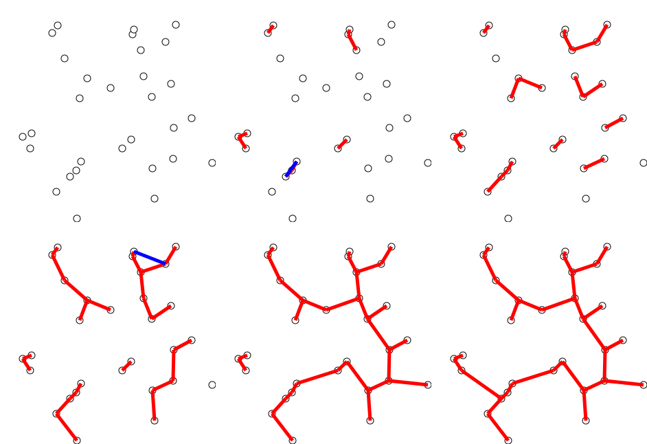
The steps of Kruskal’s algorithm:
-
Sort all the edges from smallest to largest.
-
Add the smallest edge to the final spanning tree. If adding the edge creates a cycle, move onto the next edge.
-
Keep adding all edges until all the nodes are a part of the tree.

Kruskal’s algorithm by Shiyu Ji - Own work, CC BY-SA 4.0,.
Kruskal’s algorithm is essentially the same as the Single Linkage Clustering method which results in a hierarchical dendrogram. However, with the MST the aim is to display the links between elements as opposed to clusters.
Kruskal’s algorithm is commonly implemented with a disjoint set data structure:
Kruskals(G):

# spanning tree to be returned A
A = ∅

For each vertex v ∈ G.V:
    MAKE-SET(v) # every vertex in its own set

For each edge (u, v) ∈ G.E ordered by increasing order by weight(u, v):
    if FIND-SET(u) ≠ FIND-SET(v): # if u and v aren't in the same set
        A = A ∪ {(u, v)} # add the edge to A
        # merge the set containing u and the set containing v
        UNION(u, v)

return A
More information on Kruskal’s and Prim’s algorthms can be found in the book “Introduction to algorithms” (2009) by Cormen, Leiserson, Rivest and Stein.
Prim’s Algorithm
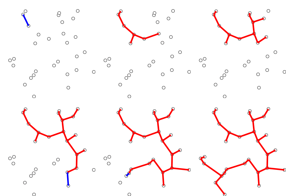
The steps for Prim’s algorithm are:
Choose and visit an arbitrary node.
-
Of all the edges from visited, pick the smallest and add the edge to the tree.
-
Keep adding edges, until all nodes are visited.

Prim’s algorithm by Shiyu Ji - Own work, CC BY-SA 4.0,.
Prim’s algorithm is recommended from a 100 vertices upwards for better time complexity (Huang et al 2009). Compared to Kruskal’s, Prim’s does not calculate all the edges from shortest to largest, instead growing from a starting node, making it more time-efficient for bigger data sets.
T = ∅; # T is the mst for final output

U = { 1 }; # U is set of visited nodes

while (U ≠ V)
    let (u, v) be the lowest cost edge such that u ∈ U and v ∈ V - U;
    T = T ∪ {(u, v)}
    U = U ∪ {v}

return T
By default the generate_mst_server method uses Kruskal’s algorithm. To use Prim’s algorithm instead, pass the parameter mst_algorithm=’prim’ into the generate_mst_server method. The documentation for generate_mst_server can be found on the Visualisations section.
MST with Custom Matrix
To create a MST visualisation, it is best to use the Visualisations methods. The generate_mst_server takes in a dataframe of log returns and returns a server. However, if you would like to input a custom matrix instead of a distance matrix, please read the information below.
To create an MST visualisation, you must input a matrix into the MST class. The DashGraph class then takes in a MST as input and returns a server.
Implementation
- class MST(matrix, matrix_type, mst_algorithm='kruskal')
-
MST is a subclass of Graph which creates a MST Graph object.
- __init__(matrix, matrix_type, mst_algorithm='kruskal')
-
Creates a MST Graph object and stores the MST inside graph attribute.
- Parameters:
-
-
matrix – (pd.DataFrame) Input matrices such as a distance or correlation matrix.
-
matrix_type – (str) Name of the matrix type (e.g. “distance” or “correlation”).
-
mst_algorithm – (str) Valid MST algorithm types include ‘kruskal’, ‘prim’, or ‘boruvka’. By default, MST algorithm uses Kruskal’s.
-
- __weakref__
-
list of weak references to the object (if defined)
- static create_mst(matrix, algorithm='kruskal')
-
This method converts the input matrix into a MST graph.
- Parameters:
-
-
matrix – (pd.DataFrame) Input matrix.
-
algorithm – (str) Valid MST algorithm types include ‘kruskal’, ‘prim’, or ‘boruvka’. By default, MST algorithm uses Kruskal’s.
-
- get_difference(input_graph_two)
-
Given two Graph with the same nodes, return a set of differences in edge connections.
- Parameters:
-
input_graph_two – (Graph) A graph to compare self.graph against.
- Returns:
-
(List) A list of unique tuples showing different edge connections.
- get_graph()
-
Returns the Graph stored as an attribute.
- Returns:
-
(nx.Graph) Returns a NetworkX graph object.
- get_graph_plot()
-
Returns the graph of the MST with labels. Assumes that the matrix contains stock names as headers.
- Returns:
-
(AxesSubplot) Axes with graph plot. Call plt.show() to display this graph.
- get_matrix_type()
-
Returns the matrix type set at initialisation.
- Returns:
-
(str) String of matrix type (eg. “correlation” or “distance”).
- get_node_colours()
-
Returns a map of industry group matched with list of nodes.
- Returns:
-
(Dict) Dictionary of industry name to list of node indexes.
- get_node_sizes()
-
Returns the node sizes as a list.
- Returns:
-
(List) List of numbers representing node sizes.
- get_pos()
-
Returns the dictionary of the nodes coordinates.
- Returns:
-
(Dict) Dictionary of node coordinates.
- set_node_groups(industry_groups)
-
Sets the node industry group, by taking in a dictionary of industry group to a list of node indexes.
- Parameters:
-
industry_groups – (Dict) Dictionary of the industry name to a list of node indexes.
- set_node_size(market_caps)
-
Sets the node sizes, given a list of market cap values corresponding to node indexes.
- Parameters:
-
market_caps – (List) List of numbers corresponding to node indexes.
MST Algorithms
When you initialise the MST object, the mst is generated and stored as attribute an self.graph. Kruskal’s algorithms is used as a default.
mst_graph = MST(custom_matrix, 'custom')
To use Prim’s algorithm, pass the string ‘prim’. Take a look below at the initialization method __init__ to see how the algorithm is set.
mst_graph = MST(custom_matrix, 'custom', 'prim')
Example Code
# Import packages
import pandas as pd

# Import MST class
from mlfinlab.networks.mst import MST

# Import Dash Graph class
from mlfinlab.networks.dash_graph import DashGraph

# Import Codependence Matrix
from mlfinlab.codependence.codependence_matrix import get_distance_matrix

# Import file containing stock log returns
url = "https://raw.githubusercontent.com/hudson-and-thames/example-data/main/logReturns.csv"
# Need to make sure all other columns are removed and leave numerical data only
log_return_dataframe = pd.read_csv(url, index_col='Date')

# Create a smaller sample for testing
log_return_dataframe = log_return_dataframe.loc[:, ['NVDA', 'TWTR', 'MSFT', 'JNJ', 'TSLA', 'GE']]

# Create your custom matrix
correlation_matrix = log_return_dataframe.corr(method='pearson')

# Create your custom matrix
custom_matrix = get_distance_matrix(correlation_matrix, metric='angular')

# Creates MST graph class objects from custom input matrix
graph = MST(custom_matrix, 'custom')

# Create and get the server
dash_graph = DashGraph(graph)
server = dash_graph.get_server()

# Run server
server.run_server()
Customizing the Graphs
To further customize the MST when it is displayed in the UI, you can add colours and change the sizes to represent for example industry groups and market cap of stocks. These features are optional.
Adding Colours to Nodes
The colours can be added by passing a dictionary of group name to list of node names corresponding to the nodes input. You then pass the dictionary to the set_node_groups method.
# Optional - add industry groups for node colour
industry = {"tech": ['NVDA', 'TWTR', 'MSFT'], "utilities": ['JNJ'], "automobiles": ['TSLA', 'GE']}
graph.set_node_groups(industry)
Adding Sizes to Nodes
The sizes can be added in a similar manner, via a list of numbers which correspond to the node indexes. The UI of the graph will then display the nodes indicating the different sizes.
# Optional - adding market cap for node size
market_caps = [2000, 2500, 3000, 1000, 5000, 3500]
graph.set_node_size(market_caps)
Research Notebook
The following notebook provides a more detailed exploration of the MST creation.
MST visualisation