Volatility Estimators
In finance, volatility (usually denoted by \(\sigma\)) is the degree of variation of a trading price series over time, usually measured by the standard deviation of logarithmic returns. Volatility is an essential metric for trading, including short-term day trading and swings trading, in which the primary focus is on daily and weekly price movements. In fact, volatility estimates can provide a profit opportunity by identifying swings and helping with bet and portfolio sizing. In order to find an edge in option trading, we need an estimate of future realized volatility to trade against that implied by the options. There are two types of volatility, historic volatility and implied volatility. Historic volatility measures a time series of past market prices, whereas implied volatility looks forward in time, being derived from the market price of a market-traded derivative (in particular, an option). But before we can forecast future volatility we need to be able to measure what it has been in the past thanks to different historic volatility estimators. These methods use some or all of the usually available daily prices that characterize a traded security: open (O), high (H), low (L), and close (C). The most common method used to estimate the historical volatility is the close-to-close method. In this approach, the historical volatility is defined as either the annualized variance or standard deviation of log returns.
where \(x_{\mathrm{i}}\) are the logarithmic returns, \(\bar{x}\) is the mean return in the sample and N is the sample size.
Many different methods have been developed to estimate the historical volatility.
Note
Underlying Literature
- The following sources elaborate extensively on the topic:
-
-
Volatility trading, Chapter 2 by Euan Sinclair.
-
Advances in Financial Machine Learning, Chapter 19 by Marcos Lopez de Prado.
-
Note
Please use data sets with columns: “open”, “high”, “low” and “close” in that order for each of the volatility estimators. Yahoo Finance needs to be installed as a pre-requisite to all the examples.
Parkinson Estimator
In 1980, Parkinson introduced the first advanced volatility estimator based only on high and low prices (HL), which can be daily, weekly, monthly, or other. Parkinson estimator is five times more efficient than the close-to-close volatility estimator as it would need fewer time periods to converge to the true volatility as it uses two prices from each period instead of just one as with the close-to-close estimator. A slightly different versions of the estimator are present in the literature. According to Sinclair, Parkinson estimator is defined as:
where \(h_{\mathrm{i}}\) is the high price in the trading period and \(l_{\mathrm{i}}\) is the low price.
According to De Prado, the estimator can be defined as:
where \(k_{1}=4 \log [2]\), \(H_{\mathrm{t}}\) is the high price for bar t, and \(L_{\mathrm{t}}\) is the low price for bar t.
The limitation of this estimator is that prices are only sampled discretely because markets are only open for part of the day. This means that the unobservable true price may not make a high or a low when we can actually measure it, hence Parkison estimator will systematically underestimate volatility.
Implementation
The following function implemented in MlFinLab can be used to derive Parkinson volatility estimator.
- parkinson(price: DataFrame, window: int, alternative_calculation=False) Series
-
Calculate volatility according to Parkinson estimator (Parkinson, 1980).
References:
Parkinson, Michael H. “The Extreme Value Method for Estimating the Variance of the Rate of Return.” The Journal of Business 53 (1980): 61-65.
Sinclair, E. (2008) Volatility Trading. John Wiley & Sons, Hoboken, NJ.
Lopez de Prado, M. (2018) Advances in Financial Machine Learning. New York, NY: John Wiley & Sons.
- Parameters:
-
-
price – (pd.DataFrame) A pandas Dataframe consisting of open, high, low and close prices of the day.
-
window – (int) Number of days in the trading period.
-
alternative_calculation – (bool) Optional. When
True, calculate the Parkinson estimator using Marcos Lopez de Prado’s formula (Lopez De Prado, 2018). WhenFalse, calculate using Sinclair’s formula (Sinclair, 2008).
-
- Returns:
-
(pd.Series) Series containing daily volatility measure according to Parkinson estimator.
Examples
The following example shows how the above functions can be used:
>>> import pandas as pd
>>> import yfinance as yf
>>> from mlfinlab.features.volatility_estimators import parkinson
>>> # Retrieve the DataFrame with time series of returns
>>> ohlc = pd.read_csv(
...     "https://raw.githubusercontent.com/hudson-and-thames/example-data/main/yahoo_finance_SPY_2012-03-26_to_2023-12-06.csv",
...     parse_dates=[0],
...     index_col=0,
... )
>>> ohlc.columns = [
...     col.lower() for col in ohlc.columns
... ]  # volatility estimators expect lower-case column names
>>> list(ohlc.columns)
['open', 'high', 'low', 'close', 'adj close', 'volume']
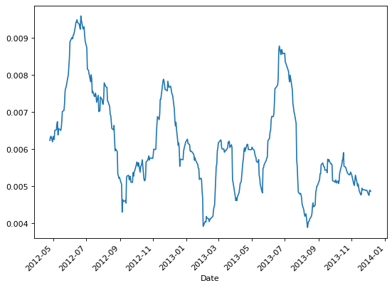
>>> # Calculate volatility with Parkinson estimator (Sinclair formula)
>>> parkinson_sinclair = parkinson(ohlc, 22, False)
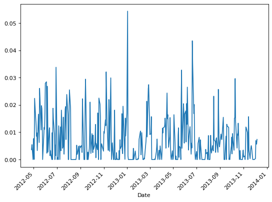
>>> # Calculate volatility with Parkinson estimator (De Prado formula)
>>> parkinson_deprado = parkinson(ohlc, 22, True)
Garman-Klass Estimator
Garman and Klass proposed in 1980 a volatility estimator that aimed to extend Parkinson’s volatility by using not only the high and low but also the opening and closing prices. During their research, Garman and Klass realized that markets are most active during the opening and closing of a trading session. Furthermore, they assumed the price change process is a geometric Brownian motion with continuous diffusion. Given these assumptions, Garman-Klass estimator is defined as:
where \(h_{\mathrm{i}}\) is the high price, \(l_{\mathrm{i}}\) is the low price and \(c_{\mathrm{i}}\) is the closing price in the trading period.
The Garman-Klass volatility estimator tries to make the best use of the commonly available price information and as such is up to eight time more efficient than the close-to-close volatility estimator. However, like Parkinson estimator, the Garman Klass estimator also provides a biased estimate of volatility as its discrete sampling doesn’t allow to take into account opening jumps in price and trend movements.
Implementation
The following function implemented in MlFinLab can be used to derive Garman-Klass volatility estimator.
- garman_klass(price: DataFrame, window: int) DataFrame
-
Calculate volatility according to Garman and Klass estimator (Garman and Klass, 1980; Sinclair, 2008).
References:
Garman, M. B., and M. J. Klass. 1980. “On the Estimation of Security Price Volatilities from Historical Data.” Journal of Business 53:67–78.
Sinclair, E. (2008) Volatility Trading. John Wiley & Sons, Hoboken, NJ.
- Parameters:
-
-
price – (pd.DataFrame) A pandas Dataframe consisting of open, high, low, close prices of the day.
-
window – (int) Number of days in the trading period.
-
- Returns:
-
(pd.Dataframe) Dataframe with daily volatility measure according to Garman-Klass estimator.
Examples
The following example shows how the above functions can be used:
>>> import pandas as pd
>>> import yfinance as yf
>>> from mlfinlab.features.volatility_estimators import garman_klass
>>> # Retrieve the dataframe with time series of returns
>>> ohlc = pd.read_csv(
...     "https://raw.githubusercontent.com/hudson-and-thames/example-data/main/yahoo_finance_SPY_2012-03-26_to_2023-12-06.csv",
...     parse_dates=[0],
...     index_col=0,
... )
>>> ohlc.columns = [
...     col.lower() for col in ohlc.columns
... ]  # volatility estimators expect lower-case column names
>>> list(ohlc.columns)
['open', 'high', 'low', 'close', 'adj close', 'volume']
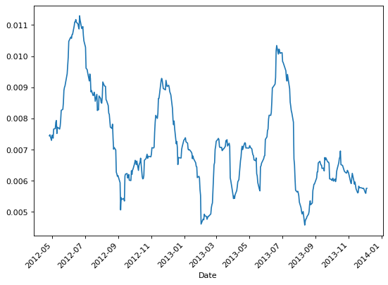
>>> # Calculate volatility with Garman-Klass estimator
>>> garman_klass_volatility = garman_klass(ohlc, window=22)
Rogers-Satchell Estimator
Volatility estimators like Parkinson’s and Garman-Klass have been shown to be more efficient than the close-to-close volatility estimator. However, these estimators assume that the underlying process follows a geometric Brownian motion with zero drift, which isn’t always the case in real markets. Particularly, during periods when the asset trends strongly, these estimators then overestimate volatility. From this observation, Rogers and Satchell proposed in 1991 a new estimator that allows for non zero drift:
where \(h_{\mathrm{i}}\) is the high price, \(l_{\mathrm{i}}\) is the low price, \(o_{\mathrm{i}}\) is the opening price and \(c_{\mathrm{i}}\) is the closing price in the trading period.
The main advantage of the Rogers-Satchell estimator is that it provides better volatility estimates during periods when the asset trends strongly. The main limitation of this estimator is the discrete sampling that doesn’t allow to take into account opening jumps in price.
Implementation
The following function implemented in MlFinLab can be used to derive Rogers-Satchell volatility estimator.
- rogers_satchell(price: DataFrame, window: int) Series
-
Calculate volatility according to Rogers and Satchell estimator (Roger and Satchell 1994, Sinclair 2008).
References:
Rogers, L., S. Satchell, and Y. Yoon. 1994. “Estimating the Volatility of Stock Prices: A Comparison of Methods that Use High and Low Prices.” Applied Financial Economics 4:241–247.
Sinclair, E. (2008) Volatility Trading. John Wiley & Sons, Hoboken, NJ.
- Parameters:
-
-
price – (pd.DataFrame) A pandas Dataframe consisting of open, high, low, close prices of the day.
-
window – (int) Number of days in the trading period.
-
- Returns:
-
(pd.Series) Series with daily volatility measure according to Rogers-Satchell estimator.
Examples
The following example shows how the above functions can be used:
>>> import pandas as pd
>>> import yfinance as yf
>>> from mlfinlab.features.volatility_estimators import rogers_satchell
>>> # Retrieve the dataframe with time series of returns
>>> df = pd.read_csv(
...     "https://raw.githubusercontent.com/hudson-and-thames/example-data/main/yahoo_finance_SPY_2012-03-26_to_2023-12-06.csv",
...     parse_dates=[0],
...     index_col=0,
... )
>>> df.columns = [
...     col.lower() for col in df.columns
... ]  # volatility estimators expect lower-case column names
>>> list(df.columns)
['open', 'high', 'low', 'close', 'adj close', 'volume']
>>> # Select open, high, low and close prices
>>> ohlc = df[["open", "high", "low", "close"]]
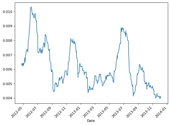
>>> # Calculate volatility with Rogers-Satchell estimator
>>> rogers_satchell_volatility = rogers_satchell(ohlc, window=20)
Yang-Zhang Estimator
Yang Zhang estimator is a volatility estimator that allows to overcome the main limitation of Parkinson’s, Garman-Klass’s and Rogers-Satchell’s estimators, that being the existing bias due to the discrete sampling as it doesn’t account for the opening jumps in price. In fact, Yang Zhang devised an estimator that combines the classical and Rogers-Satchell estimator, showing that it has the minimum variance and is both unbiased and independent of process drift and opening gaps. The Yang Zhang estimator is given as (from the original paper):
where
where \(h_{\mathrm{i}}\) is the high price, \(l_{\mathrm{i}}\) is the low price, \(o_{\mathrm{i}}\) is the opening price and \(c_{\mathrm{i}}\) is the closing price in the trading period.
The efficiency of Yang-Zhang estimator has a peak value of 14, meaning that using only two days’ data for this estimator gives the same accuracy as the classical estimator using three week’s data. However, where the process is dominated by opening jumps the efficiency reduces to almost one, which means there is no improvement over the classical clos-to-close estimator.
Note
Yang-Zhang Estimator
There is a slight difference between the formulas presented in the orginal paper, “Drift-Independent Volatility Estimation Based on High, Low, Open, and Close Prices, (Yang, D., and Q. Zhang. 2000)” and the book Volatility Trading (Sinclair, E. 2008) . Our implementation uses the original paper as reference.
Implementation
The following function implemented in MlFinLab can be used to derive Yang-Zhang volatility estimator.
- yang_zhang(price: DataFrame, window: int) Series
-
Calculate volatility according to Yang and Zhang estimator
- Parameters:
-
-
price – (pd.DataFrame) A pandas Dataframe with columns of
open,high,low, andclose, each containing the daily open, high, low and close prices, respectively. -
window – (int) Number of days in the trading period.
-
- Returns:
-
(pd.Series) Series with daily volatility measure according to Yang-Zhang estimator.
- References:
-
-
Yang, D., and Q. Zhang. 2000. “Drift-Independent Volatility Estimation Based on High, Low, Open, and Close Prices.” Journal of Business 73:477–491.
-
Sinclair, E. (2008) Volatility Trading. John Wiley & Sons, Hoboken, NJ.
-
Examples
The following example shows how the above functions can be used:
>>> import pandas as pd
>>> import yfinance as yf
>>> from mlfinlab.features.volatility_estimators import yang_zhang
>>> # Get the dataframe with time series of returns
>>> df = pd.read_csv(
...     "https://raw.githubusercontent.com/hudson-and-thames/example-data/main/yahoo_finance_SPY_2012-03-26_to_2023-12-06.csv",
...     parse_dates=[0],
...     index_col=0,
... )
>>> df.columns = [
...     col.lower() for col in df.columns
... ]  # volatility estimators expect lower-case column names
>>> list(df.columns)
['open', 'high', 'low', 'close', 'adj close', 'volume']
>>> # Select open, high, low and close prices
>>> ohlc = df.iloc[:, 0:4]
>>> ohlc.columns = [col.lower() for col in ohlc.columns]
>>> # Calculate volatility with Yang Zhang estimator
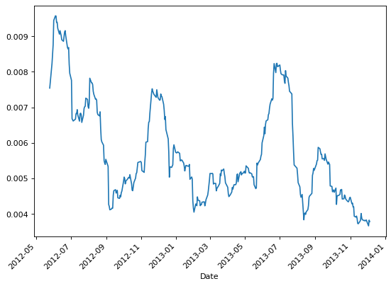
>>> yang_zhang_volatility = yang_zhang(ohlc, window=22)
Corwin-Shultz Estimator
Corwin-Schultz is a bid-ask spread estimator from daily high and low prices to measure the bid-ask spread of shares, using the formula:
where
The estimator is based on the assumption that daily high prices are typically buyer initiated and low prices are seller initiated, and therefore the ratio of high-to-low prices for a day reflects both the fundamental volatility of stock and its bid-ask spread. Furthermore, it assumes that the volatility component of the high-to-low price ratio increases proportionately with the length of trading interval whereas the component due to bid-ask spreads does not. Corwin-Schultz estimation bias and the frequency of negative estimates increase in liquid assets or when price volatility is high.
Implementation
The following function implemented in MlFinLab can be used to derive Corwin-Shultz estimator.
- CorwinShultzVolatility(price: DataFrame, window: int)
-
A class that allows to calculate the alpha, beta and gamma parameters as well as the spread according to Corwin and Schultz estimator (Corwin and Schultz 2012, Lopez de Prado 2018).
References:
CORWIN, S.A. and SCHULTZ, P. (2012), A Simple Way to Estimate Bid-Ask Spreads from Daily High and Low Prices. The Journal of Finance, 67: 719-760
Lopez de Prado, M. (2018) Advances in Financial Machine Learning. New York, NY: John Wiley & Sons.
Examples
The following example shows how the above functions can be used:
>>> import pandas as pd
>>> import yfinance as yf
>>> from mlfinlab.features.volatility_estimators import CorwinShultzVolatility
>>> # Retrieve the dataframe with time series of returns
>>> ohlc = pd.read_csv(
...     "https://raw.githubusercontent.com/hudson-and-thames/example-data/main/yahoo_finance_SPY_2012-03-26_to_2023-12-06.csv",
...     parse_dates=[0],
...     index_col=0,
... )
>>> ohlc.columns = [
...     col.lower() for col in ohlc.columns
... ]  # volatility estimators expect lower-case column names
>>> list(df.columns)
['open', 'high', 'low', 'close', 'adj close', 'volume']
>>> # Calculate volatility with Corwin Shultz estimator
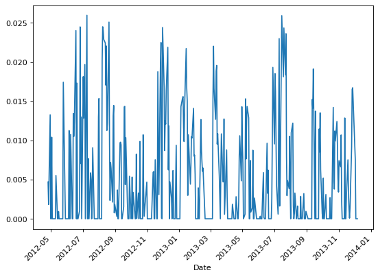
>>> corwin_shultz_temp = CorwinShultzVolatility(ohlc, 22)
>>> corwin_shultz_volatility = corwin_shultz_temp.calculate_volatility()
Cho-Frees Estimator
Cho Frees estimator is a volatility estimator which eliminates, at least asymptotically, the biases that are caused by the discreteness of observed stock prices. Assuming that the observed prices are continuously monitored, using the notion of how quickly the price changes rather than how much the price changes an estimator is constructed:
where \(\delta=\log (1+d)\) being d a known constant (1/8 for the New York Stock Exchange for example), \(\hat{\mu}=\bar{\tau}_{n}^{-1} \log \left(P\left(\tau_{n}\right)\right)\) and \(\bar{\tau}_{n}=\tau_{n} / n\).
It is shown that this estimator has desirable asymptotic properties, including consistency and normality. Also, it outperforms natural estimators for low and middle-priced stocks. Further, simulation studies demonstrate that the proposed estimator is robust to certain misspecifications in measuring the time between price changes.
Implementation
The following function implemented in MlFinLab can be used to derive Cho-Frees estimator.
- cho_frees(price: DataFrame, delta: float) DataFrame
-
Calculate volatility according temporal estimator (Cho D. & Frees, 1988).
References:
D. Cho and E. Frees. “Estimating the Volatility of Discrete Stock Prices.” Working paper, University of Wisconsin-Madison, 1986.
- Parameters:
-
-
price – (pd.DataFrame) A pandas DataFrame consisting of a
DatetimeIndexand close prices of the day in a ‘close’ column. -
delta – (float) A number for defining the wide of the barrier for exiting.
-
- Returns:
-
(pd.Dataframe) Dataframe with daily volatility measure according to First Exit Times estimator.
Examples
The following example shows how the above functions can be used:
>>> import pandas as pd
>>> import yfinance as yf
>>> from mlfinlab.features.volatility_estimators import cho_frees
>>> # Retrieve the dataframe with time series of returns
>>> ohlc = pd.read_csv(
...     "https://raw.githubusercontent.com/hudson-and-thames/example-data/main/yahoo_finance_SPY_2012-03-26_to_2023-12-06.csv",
...     parse_dates=[0],
...     index_col=0,
... )
>>> ohlc.columns = [col.lower() for col in ohlc.columns]  # volatility estimators expect lower-case column names
>>> list(df.columns)
['open', 'high', 'low', 'close', 'adj close', 'volume']
>>> # Calculate volatility with Cho Frees estimator
>>> cho_frees_volatility = cho_frees(ohlc, 0.01)

First Exit Time Estimator
The first exit times estimator is a volatility estimator that derives from Cho Frees estimator, and as the latter, it considers how quickly the price changes rather than how much the price changes. The estimator is constructed by considering a price corridor, \(\Delta\) up and \(\Delta\) down from the initial spot price. Each time the upper or lower barrier of the corridor is touched, the barrier is reset around the current price, and the times to reach the barrier noted form a sequence of exit times from which the volatility is estimated using the formula:
where \(E[\tau]\)is the sample mean of the hitting times after n observations. We don’t know the true value of \(E[\tau]\) : We can only make estimates based on the observed data. So the sampling distribution of \(\tau\) is important. The true value will be slightly lower than the naive estimate due to Jensen’s inequality. That is,
But it is possible to make a second order correction that adjusts for the variance of \(\tau\).
If \(\bar{\tau}\) is the mean of the sample of the \(n\) first exit times we have, by the Central Limit Theorem,
Our goal is to derive an unbiased estimator of the population variance, To do this we define a new random variable \(\delta \tau\) by
This is a random variable with zero mean and a variance, \(\operatorname{Var}(\tau) / n\). Now define a function, \(f\).
The sample volatility derived with this formula is biased unless n is large, therefore we can derive the unbiased volatility by considering this relationship between the two:
where \(E[f(\bar{\tau})]\)is the sample biased volatility, and \(\sigma\) is the unbiased volatility.
This estimator assumes Brownian motion for the log-price process and a negligible drift in prices, hence its estimates may be biased in periods of time during which prices trends significantly.
Implementation
The following function implemented in MlFinLab can be used to derive the first exit times estimator.
- first_exit_times(price: DataFrame, delta: float, window: int) DataFrame
-
Calculate volatility according First Exit Times estimator (Sinclair, 2008).
References:
Sinclair, E. (2008) Volatility Trading. John Wiley & Sons, Hoboken, NJ.
- Parameters:
-
-
price – (pd.DataFrame) A pandas DataFrame consisting of a
DatetimeIndexand close prices of the day in a ‘close’ column. -
delta – (float) A number for defining the wide of the barrier for exiting.
-
window – (int) Sliding window used in calculations.
-
- Returns:
-
(pd.Dataframe) Dataframe with daily volatility measure according to First Exit Times estimator.
Examples
The following example shows how the above functions can be used:
>>> import pandas as pd
>>> import yfinance as yf
>>> from mlfinlab.features.volatility_estimators import first_exit_times
>>> # Getting the dataframe with time series of returns
>>> ohlc = pd.read_csv(
...     "https://raw.githubusercontent.com/hudson-and-thames/example-data/main/yahoo_finance_SPY_2012-03-26_to_2023-12-06.csv",
...     parse_dates=[0],
...     index_col=0,
... )
>>> ohlc.columns = [
...     col.lower() for col in ohlc.columns
... ]  # volatility estimators expect lower-case column names
>>> list(df.columns)
['open', 'high', 'low', 'close', 'adj close', 'volume']
>>> # Calculating volatility with first exit times estimator
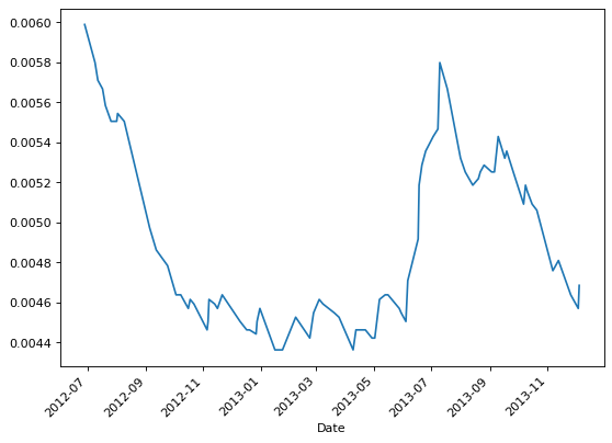
>>> first_exit_times_volatility = first_exit_times(ohlc, 0.01, 22)
>>> first_exit_times_volatility.tail()
Date...
2013-11-07...0.004...
Research Notebook
The following research notebook can be used to better understand the volatility estimators.