Third Generation Models

Third generation models look at microstructures through the lens of randomly selected traders that arrive at the market sequentially and independently. Sequential trade models have become very popular among market makers. One reason is, they incorporate the sources of uncertainty faced by liquidity providers, namely the probability that an informational event has taken place, the probability that such event is negative, the arrival rate of noise traders, and the arrival rate of informed traders. With those variables, market makers must update quotes dynamically, and manage their inventories.

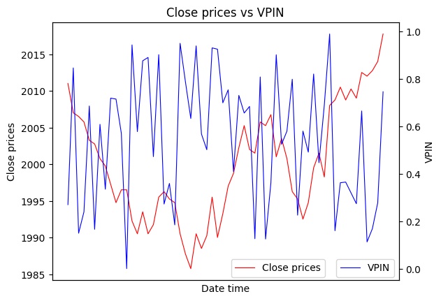
Closing prices in red, and VPIN in blue

Note

Underlying Literature

The following sources elaborate extensively on the topic:

• Advances in Financial Machine Learning, Chapter 19, Section 5 by Marcos Lopez de Prado. Describes the emergence and modern day uses of the second generation of microstructural features in more detail

---

Probability of Information-based Trading

The following description is based on Section 19.5.1 of Advances in Financial Machine Learning:

” Easley et al. (1998) use trade data to determine the probability of information-based trading (PIN) of individual securities. This microstructure model views trading as a game between market makers and position takers that is repeated over multiple trading periods.

Denote a security’s price as \(S\), with present value \(S_{0}\). However, once a certain amount of new information has been incorporated into the price, \(S\) will be either \(S_{B}\) (bad news) or \(S_{G}\) (good news). There is a probability \(\alpha\) that new information will arrive within the timeframe of the analysis, a probability \(\delta\) that the news will be bad, and a probability \((1-\delta)\) that the news will be good. These authors prove that the expected value of the security’s price can then be computed at time \(t\) as

\[\mathrm{E}\left[S_{t}\right]=\left(1-\alpha_{t}\right) S_{0}+\alpha_{t}\left[\delta_{t} S_{B}+\left(1-\delta_{t}\right) S_{G}\right]\]

Following a Poisson distribution, informed traders arrive at a rate \(\mu\), and uninformed traders arrive at a rate \(\varepsilon\). Then, in order to avoid losses from informed traders, market makers reach breakeven at a bid level \(B_{t}\),

\[\mathrm{E}\left[B_{t}\right]=\mathrm{E}\left[S_{t}\right]-\frac{\mu \alpha_{t} \delta_{t}}{\varepsilon+\mu \alpha_{t} \delta_{t}}\left(\mathrm{E}\left[S_{t}\right]-S_{B}\right)\]

and the breakeven ask level \(A_{t}\) at time t must be,

\[\mathrm{E}\left[A_{t}\right]=\mathrm{E}\left[S_{t}\right]+\frac{\mu \alpha_{t}\left(1-\delta_{t}\right)}{\varepsilon+\mu \alpha_{t}\left(1-\delta_{t}\right)}\left(S_{G}-\mathrm{E}\left[S_{t}\right]\right)\]

It follows that the breakeven bid-ask spread is determined as

\[\mathrm{E}\left[A_{t}-B_{t}\right]=\frac{\mu \alpha_{t}\left(1-\delta_{t}\right)}{\varepsilon+\mu \alpha_{t}\left(1-\delta_{t}\right)}\left(S_{G}-\mathrm{E}\left[S_{t}\right]\right)+\frac{\mu \alpha_{t} \delta_{t}}{\varepsilon+\mu \alpha_{t} \delta_{t}}\left(\mathrm{E}\left[S_{t}\right]-S_{B}\right)\]

For the standard case when \(\delta_{t}=\frac{1}{2}\), we obtain

\[\delta_{t}=\frac{1}{2} \Rightarrow \mathrm{E}\left[A_{t}-B_{t}\right]=\frac{\alpha_{t} \mu}{\alpha_{t} \mu+2 \varepsilon}\left(S_{G}-S_{B}\right)\]

This equation tells us that the critical factor that determines the price range at which market makers provide liquidity is

\[P I N_{t}=\frac{\alpha_{t} \mu}{\alpha_{t} \mu+2 \varepsilon}\]

The subscript \(t1\) indicates that the probabilities \(\alpha\) and \(\delta\) are estimated at that point in time. The authors apply a Bayesian updating process to incorporate information after each trade arrives to the market. In order to determine the value \(P I N_{t}\), we must estimate four non-observable parameters, namely \(\{\alpha, \delta, \mu, \varepsilon\}\). A maximum-likelihood approach is to fit a mixture of three Poisson distributions,

where \(V^{B}\) is the volume traded against the ask (buy-initiated trades), and \(V^{S}\) is the volume traded against the bid (sell-initiated trades).”

---

Volume-Synchronized Probability of Informed Trading

The following description is based on Section 19.5.2 of Advances in Financial Machine Learning:

” Easley et al. (2008) proved that

\[\begin{split}\begin{aligned} \mathrm{E}\left[V^{B}-V^{S}\right] &=(1-\alpha)(\varepsilon-\varepsilon)+\alpha(1-\delta)(\varepsilon-(\mu+\varepsilon))+\alpha \delta(\mu+\varepsilon-\varepsilon) \\ &=\alpha \mu(1-2 \delta) \end{aligned}\end{split}\]

and in particular, for a sufficiently large \(\mu\),

\[\mathrm{E}\left[\left|V^{B}-V^{S}\right|\right] \approx \alpha \mu\]

Easley et al. (2011) proposed a high-frequency estimate of PIN, which they named volume-synchronized probability of informed trading (VPIN). This procedure adopts a volume clock, which synchronizes the data sampling with market activity, as captured by volume. We can then estimate

\[\frac{1}{n} \sum_{\tau=1}^{n}\left|V_{\tau}^{B}-V_{\tau}^{S}\right| \approx \alpha \mu\]

where \(V_{\tau}^{B}1\) is the sum of volumes from buy-initiated trades within volume bar \(\tau, V_{\tau}^{S}\) is the sum of volumes from sell-initiated trades within volume bar \(\tau\), and \(n\) is the number of bars used to produce this estimate. Because all volume bars are of the same size, \(V\), we know that by construction

\[\frac{1}{n} \sum_{\tau=1}^{n}\left(V_{\tau}^{B}+V_{\tau}^{S}\right)=V=\alpha \mu+2 \varepsilon\]

Hence, PIN can be estimated in high-frequency as

\[\operatorname{VPIN}_{\tau}=\frac{\sum_{\tau=1}^{n}\left|V_{\tau}^{B}-V_{\tau}^{S}\right|}{\sum_{\tau=1}^{n}\left(V_{\tau}^{B}+V_{\tau}^{S}\right)}=\frac{\sum_{\tau=1}^{n}\left|V_{\tau}^{B}-V_{\tau}^{S}\right|}{n V} "\]

Implementation

Third generation models implementation (VPIN).

get_vpin(volume: Series, buy_volume: Series, window: int = 1) → Series

Advances in Financial Machine Learning, p. 292-293.

Get Volume-Synchronized Probability of Informed Trading (VPIN) from bars.

Parameters:

• volume – (pd.Series) Bar volume.

• buy_volume – (pd.Series) Bar volume classified as buy (either tick rule, BVC or aggressor side methods applied).

• window – (int) Estimation window.

Returns:

(pd.Series) VPIN series.

Example

>>> import pandas as pd
>>> from mlfinlab.util.volume_classifier import get_bvc_buy_volume
>>> from mlfinlab.microstructural_features.third_generation import get_vpin
>>> # Download data
>>> data = pd.read_csv(
...     "https://raw.githubusercontent.com/hudson-and-thames/example-data/main/dollar_bars.csv",
...     index_col="date_time",
... )
>>> # Get the BVC volume
>>> bvc_buy_volume = get_bvc_buy_volume(data["close"], data["cum_vol"], window=20)
>>> # Calculate the VPIN
>>> vpin = get_vpin(data.cum_vol, bvc_buy_volume)
>>> print(vpin.dropna())  
date_time
2015-01-02 16:30:52.544    0.846210
2015-01-02 16:43:33.673    0.746311...

---

Features Generator

Some microstructural features need to be calculated from trades (tick rule/volume/percent change entropies, average tick size, vwap, tick rule sum, trade based lambdas). MlFinLab has a special function which calculates features for generated bars using trade data and bar date_time index.

Implementation

Inter-bar feature generator which uses trades data and bars index to calculate inter-bar features.

class MicrostructuralFeaturesGenerator(trades_input: (<class 'str'>, <class 'pandas.core.frame.DataFrame'>), tick_num_series: ~pandas.core.series.Series, batch_size: int = 20000000.0, volume_encoding: dict | None = None, pct_encoding: dict | None = None)

Class which is used to generate inter-bar features when bars are already compressed.

Parameters:

• trades_input – (str/pd.DataFrame) Path to the csv file or Pandas DataFrame containing raw tick data in the format[date_time, price, volume].

• tick_num_series – (pd.Series) Series of tick number where bar was formed.

• batch_size – (int) Number of rows to read in from the csv, per batch.

• volume_encoding – (dict) Dictionary of encoding scheme for trades size used to calculate entropy on encoded messages.

• pct_encoding – (dict) Dictionary of encoding scheme for log returns used to calculate entropy on encoded messages.

get_features(verbose=True, to_csv=False, output_path=None)

Reads a csv file of ticks or pd.DataFrame in batches and then constructs corresponding microstructural intra-bar features: average tick size, tick rule sum, VWAP, Kyle lambda, Amihud lambda, Hasbrouck lambda, tick/volume/pct Shannon, Lempel-Ziv, Plug-in entropies if corresponding mapping dictionaries are provided (self.volume_encoding, self.pct_encoding). The csv file must have only 3 columns: date_time, price, & volume.

Parameters:

• verbose – (bool) Flag whether to print message on each processed batch or not.

• to_csv – (bool) Flag for writing the results of bars generation to local csv file, or to in-memory DataFrame.

• output_path – (bool) Path to results file, if to_csv = True.

Returns:

(DataFrame or None) Microstructural features for bar index.

Example

>>> import numpy as np
>>> import pandas as pd
>>> from mlfinlab.data_structures.standard_data_structures import get_volume_bars
>>> from mlfinlab.microstructural_features.encoding import quantile_mapping
>>> from mlfinlab.microstructural_features.feature_generator import (
...     MicrostructuralFeaturesGenerator,
... )
>>> url = "https://raw.githubusercontent.com/hudson-and-thames/example-data/main/test_tick_data.csv"
>>> df_trades = pd.read_csv(url, parse_dates=[0])
>>> df_trades = df_trades.iloc[:10000]  # Take slice to avoid look-ahead bias
>>> df_trades["log_ret"] = np.log(df_trades["Price"] / df_trades["Price"].shift(1)).dropna()
>>> non_null_log_ret = df_trades[df_trades.log_ret != 0].log_ret.dropna()
>>> # Take unique volumes only
>>> volume_mapping = quantile_mapping(df_trades["Volume"].drop_duplicates(), num_letters=10)
>>> returns_mapping = quantile_mapping(non_null_log_ret, num_letters=10)
>>> # Compress bars from ticks
>>> compressed_bars = get_volume_bars(df_trades, threshold=20, verbose=False)
>>> tick_number = compressed_bars.tick_num  # tick number where bar was formed
>>> gen = MicrostructuralFeaturesGenerator(
...     url, tick_number, volume_encoding=volume_mapping, pct_encoding=returns_mapping
... )
>>> gen.get_features(
...     to_csv=False, verbose=False
... )  
date_time...

---

Research Notebook

The following research notebooks can be used to better understand labeling excess over mean.

• Microstructural Features

Download Notebook

• Chapter 19 Microstructure Features

Download Notebook

---

Presentation Slides

Note

• pg 1-14: Structural Breaks

• pg 15-24: Entropy Features

• pg 25-37: Microstructural Features

---

References

• de Prado, M.L., 2018. Advances in financial machine learning. John Wiley & Sons.

• de Prado, M.L., 2018. Market Microstructure in the Age of Machine Learning. Available at SSRN 3193702.

• de Prado, M.L., 2018. Advances in Financial Machine Learning: Lecture 8/10 (seminar slides). Available at SSRN 3270269.

• Easley, D., O’Hara, M. and Paperman, J., 1998. Financial analysts and information-based trade. Journal of Financial Markets, 1(2), pp.175-201.

• Easley, D., De Prado, M.M.L. and O’Hara, M., 2011. The microstructure of the “flash crash”: flow toxicity, liquidity crashes, and the probability of informed trading. The Journal of Portfolio Management, 37(2), pp.118-128.